Graph-based

Graph-based Asynchronous Event Processing

1. Introduction

1. Since the output of an event camera is a sparse asynchronous events stream, most works transform events stream into:

   • regular 2D event frames
   • 3D voxel grids

   丢失了事件的稀疏性、把事件的时间戳量化

   Event-by-event processint:

   • SNN
   • Time-surface-based methods

   对调参敏感、难以训练

2. 当前基于事件的GNN仍然是分批处理事件，at the cost of discarding the low latency nature of events data.

3. Contributions

   • graph-based recursive algorithm
   • a novel incremental graph convolution
   • an event-specific radius search algorithm
     • 减少了query和insertion/deletion的时间复杂度

3. Method

3.1 Event Graph

• connectivity of nodes: radius-neighborhood graph strategy

  $v_i$ and $v_j$ are connected with an edge only if their weighted Euclidean distance less than R.

• limit the size of graph: 每个节点有最大度限制$D_{max}$

3.2 Spatial Graph Convolution

1. Spatial Graph Convolution

   Formally, it aggregates a new feature vector for each vertex using its neighborhood information weighted by a trainable kernel function.

   $$\begin{gathered} (f \otimes g)(i)=\sum_{j \in E(i)} f(j) h_{\theta}, \\ h_{\theta}=h_{\theta}\left(f(i), f(j), e_{i j}\right), \end{gathered}$$

   Eq 1.use summation as the aggregation operation
   • $h_{\theta}$ is a function determining how the features are aggregated by making use of two node features and edge attributes.
   • $f(i)$ is the node features.

4. Method

4.1 Slide Convolution

Infeasible version

update the graph by sliding new events in and sliding events out, then apply convolution on the full graph.

• 需要每次移动滑动窗口都处理整个窗口内的事件

Improved version

just compute the features around the newly active or inactive nodes.

• 但是仅能应用在单层上

slide convolution

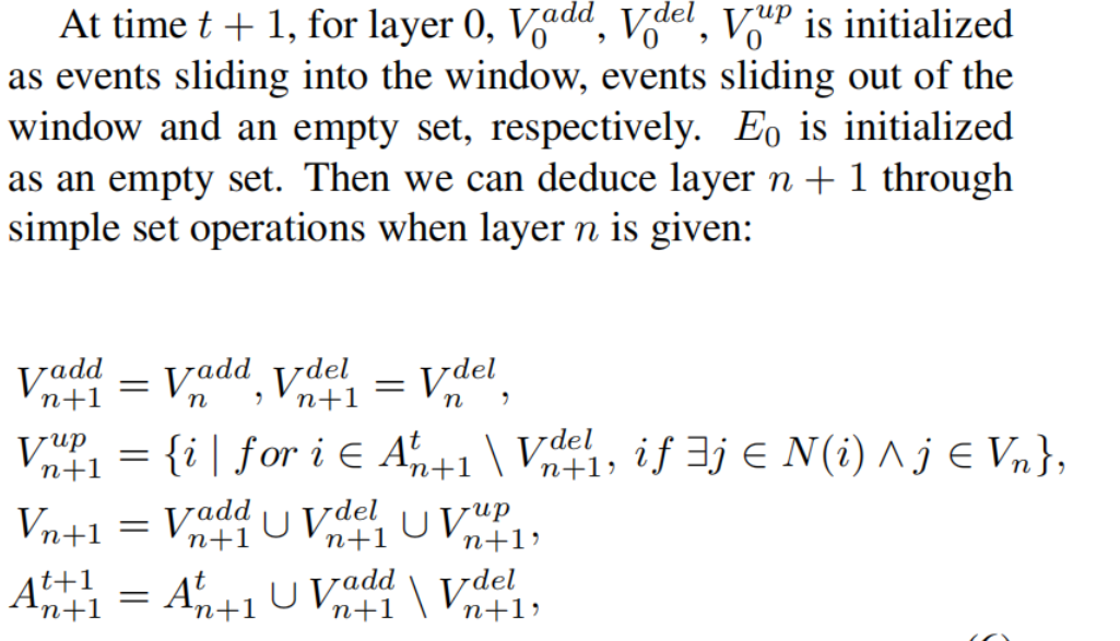
• rewrite the convolution in a multi-layer architecture

  $$f_{n+1}(i)=\sum_{j \in N(i)} f_{n}(j) h_{\theta}, \text { for } i \in A_{n+1}$$

  • $A_{n+1}$: existing set, represents all existing nodes in the graph at layer at n+1

  • $N(i)$: map that stores which nodes at layer n contribute to node i at layer $n+1$.

    Here, $N(i)$ is one-hop neighbour of node i.

• leverage the temporal sparsity of the event stream, i.e., some nodes stay same values at 2 consecutive timestamp:

  $$\begin{aligned} f_{n+1}^{t+1}(i) &=f_{n+1}^{t}(i)+\Delta_{n+1}(i) \\ \Delta_{n+1}(i) &=\sum_{(j, i) \in E_{n+1}}\left(f_{n}^{t+1}(j)-f_{n}^{t}(j)\right) h_{\theta} \end{aligned}$$

  • $E_{n+1}$: a set of directed edges containing all the edges that point to modified nodes.

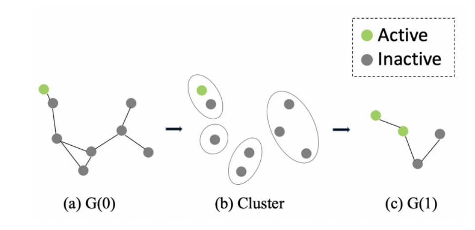
• divide nodes that need to be updated into 3 categories:

  • the ones deleted from the graph, $V^{del}$
  • the ones newly added to the graph $V^{add}$
  • the ones that locate in the receptive field $V^{up}$
  

• $V_{n+1}$ and $E_{n+1}$ is built from state at previous layer, 所以不需要记录之前的状态，依次更新过来就行。

• 但是需要维护A的之前状态

• 如何更新$f_{n+1}^t$?

  • for $V_{n+1}^{add}$, assigned to zeros
  • for $V_{n+1}^{del}$, assigned $f_{n+1}^{t+1}$ to zeros

• To extend to pooling operations

  $N(i)$: the nodes located in the same voxel($S(voxel)$)

  

4.2 Pixel Queue

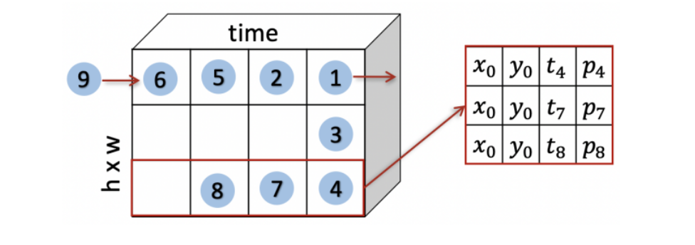
1. Pixel queue stores the most recent events at each location sorted by the time of their arrival.
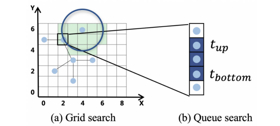
2. two-stage radius
   • For a query event（$x_0,y_0,t_0$）and the radius R, we can determine candidate pixels and corresponding queues.
   • For a candidate pixel queue with spatial offset $(\delta_x, \delta_y)$ ​ from the query event, the target evetns contained in it must have lower bound $t_0 - \sqrt{R^2 - (\delta_x^2 + \delta_y^2)}(t_{bottom})$​ and upper bound $t_0 + \sqrt{R^2 - (\delta_x^2 + \delta_y^2)}(t_{up})$​
   • 对于上下界，使用二分查找找到位于其中的事件——final query result

4.3 State-aware Module

随着事件增多，预测的结果将会逐渐变得稳定，此时没有必要继续增加更多的事件。

State-aware Module

Specifically, we use a multi-layer perceptron to represent a state-aware function which maps the graph feature map to a binary prediction.

The prediction result means whether it achieves the stable status.

在训练阶段训练MLP, 看作是事件下标的一个函数，当没有明显增加的时候认为达到稳定状态， i.e.输出1.

5. Experiment

1. Comparison to the batch-wise way

   减小batch size 减小了延迟但是会导致准确率下降

2. Trade-off between latency and computational effort

   Event-wise减小了latency，但是使得计算成本增加。