OANet

Learning Two-View Correspondences

1. Introduction

1. Until recently, most of geometric matching pipeline focus on learning local feature detectors and descriptors.

2. Previous works exploited PointNet-like architecture and Context Normalization(PointCN)

   CONS

   • apply MLP on each point individually and cannot capture the local context.

     邻居像素的也有类似的运动$\rightarrow$ 有利于outlier rejection

   • Context Normalization编码全局信息，忽略了不同点之间的特性

   One of the challenges in mitigating the limitations above:

   • sparse matches have no well-defined neighbors
   • the relation are unordered and have no stable relations to be captured.

3. draw inspiration from the hierarchical representations of GNN

   • generalize DiffPool: permutation-invariant and to capture the local context

4. threefold contributions:

   • DiffPool and DiffUnpool layers to capture the local context of unordered sparse correspondences in a learnable manner
   • Order-Aware Filtering block: exploits the complex global context of sparse correspondences.
   • accuracy$\uparrow$

2. Related work

2.2 Outlier Rejection

1. putative correspondences established by handcrafted or learned features contain many outliers.

2. RANSAC: most popular outlier rejection method

   PointCN: reformulated the outlier reection task as an inlier/outlier clasfication problem and an essential matrix regression problem

   Context Normalization: can drastically improve the performance.

3. Geometric Deep Learning deals with data on non-Euclidean domains.

   和点云不同的是，sparse correspondences have no well-defined neighbors.

3. Order-Aware Network

3.1 Formulation

GOAL: Given image pairs, remove outliers

• using features to find nearest neighbors in the other image.
• outlier rejection
• an essential matrix can be recovered

INPUT

• $$\mathbf{C}=\left[c_{1} ; c_{2} ; \ldots ; c_{N}\right] \in \mathcal{R}^{N \times 4}, c_{i}=\left(x_{1}^{i}, y_{1}^{i}, x_{2}^{i}, y_{2}^{i}\right)$$

  • $C_i$ is a correspondence and $(x_1^i, y_1^i),(x_2^i, y_2^i)$ are the coordinates of keypoints in these two images.

Architecture

• $$\begin{gathered} \mathbf{z}=f_{\phi}(\mathbf{C}) \\ \mathbf{w}=\tanh (\operatorname{ReLU}(\mathbf{z})) \\ \hat{\mathbf{E}}=g(\mathbf{w}, \mathbf{C}) \end{gathered}$$

  • Z is the logit values for classfication
  • $f_{\phi}(\cdot)$ is a permutation-equivariant neural network and $\phi$ denotes the network parameters.
  • w is the weights of correspondences.

3.2 Differentiable Pooling Layer

The unordered input correspondences require network $f_{\phi}(\cdot)$ to be permutation-equivariant, so PointNet-Like architecture was used.

• However, PointNet-like architecture has the drawback in capturing the local context because there is no direct interaction between points.

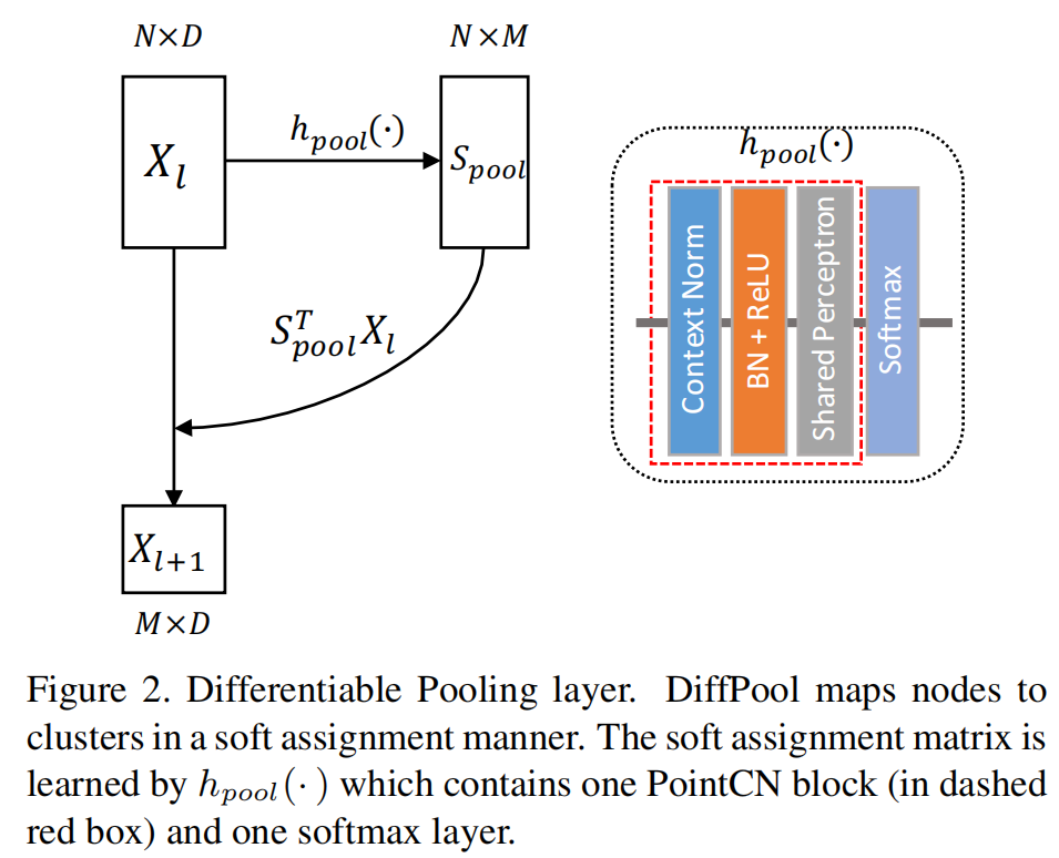
• Rather than employing a hard assignment for each node, the DiffPool layer learns a soft assignment matrix.

  $S_{pool} \in \textit{R}^{N\times M}$, Diff-Pool maps N nodes to M clusters:

  $$\mathbf{X}_{l+1}=\mathbf{S}_{\text {pool }}^{T} \mathbf{X}_{l}​$$

  

$$S_{pool} = softmax(h_{pool}(X_l))$$

• $h_{pool}(\cdot)$ is one PointCN block here.
• softmax layer is applied to normalize the assignment matrix along the row dimension.

Permutation-invariance

DiffPool is permutation-invariance:

$$\tilde{\mathbf{S}}_{\text {pool }}=\operatorname{softmax}\left(h_{\text {pool }}\left(\mathbf{P X}_{l}\right)\right)=\mathbf{P} \mathbf{S}_{\text {pool }}$$

• $P \in \{0, 1\}^{N\times N}$
• Since both $h_{pool}(\cdot)$ and softmax are permutation-equivariant functions, so

$$\mathbf{X}_{l+1}=\tilde{\mathbf{S}}_{\text {pool }}^{T} \mathbf{P X}_{l}=\mathbf{S}_{\text {pool }}^{T} \mathbf{P}^{T} \mathbf{P X}_{l}=\mathbf{S}_{\text {pool }}^{T} \mathbf{X}_{l}$$

once the network is learned, no mater how the input are permuted, they will be mapped into clusters in a particular learned canonical order

3.3 Differentiable Unpooling Layer

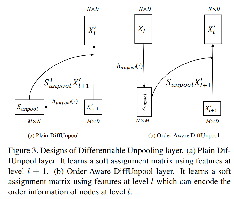
1. to upsample the coarse represention and build a hierarchical architecture.

   

   $$S_{unpool} = softmax(h_{unpool}(X_{l+1}^{'}))$$

   • 

     

   • 3(a) cannot recover the original spatial order of $X_l$​​ because of permutation-invariant operation, and $S_{unpool}$ only utilizes information at level $l+1$

   • 3(b) advise it as an Order-Aware DiffUnpool layer

     $$S_{unpool} = softmax(h_{unpool}(X_l))$$

     $$X_l^{'} = S_{unpool} X_{l+1}^{'}$$

     因为$S_{unpool}$编码了序列信息，所以学出来的$X_l^{'}$也会保持序列特征。

3.4 Order-Aware Filtering Block

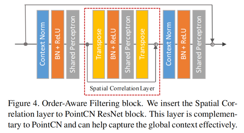
Here we propose a simple but more effective operation than PointCN block, which is called Spatial Correlation layer to explicitly model relation between different nodes and capture the complex global context.

• the weights are shared along the channel dimension

• the spatial correlation layer is orthogonal to PointCN, since one is along the spatial dimension and the other is along the channel dimension.

• Spatial Correlation layer is implemented by tranposing the spatial and channel dimensions of features.

  After the weight-sharing perceptrons layer, we transpose features back.

• Note that before the DiffPool layer, we cannot apply the Spatial Correlation layer on the feature maps as the input data is unordered and there is no stable spatial relation to be captured.